Batch trace workflow

Overview

With the Batch Trace workflow, you can trace structures in multiple images using predefined settings (configuration). Neurolucida 360 software then generates an .ASC or .DAT data file for each image processed.

Access the workflow by clicking the Batch Trace button in the Trace ribbon, Automatic section of the Main (2D) window.

The images to be processed must be set to the same µm/px scale and X/Y, and, for 3D images, to the same Z step.

Batch trace workflow steps overview and links

These are the steps in the Batch trace workflow. [Click the step to jump to instructions]

1. Choose configuration
2. Select image files
3. Specify image scaling
4. Define output settings
5. Trace all files
6. Finish

Before you start—Save 3D settings

1. In the 3D environment, open an image stack representative of the image stacks you'll process with the batch run.
2. Adjust settings, then detect somas and trace trees with the automatic method.
3. Click the 3D Settings button to save the settings used in the previous step. They will be available for use in the Batch Trace workflow.
4. In the 3D Settings window, click Save current settings and enter a name for the configuration.
5. Close the 3D window. You don't need to save the data file.
6. In the 2D window, go to the Trace ribbon and click the Batch trace button in the Automatic section to start the workflow.

Workflow steps

1. Choose configuration

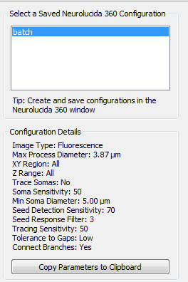
   1. Select the configuration or "3D Settings" from the list (the configuration was previously created and saved in the 3D window with an image stack representative of the image stacks to be processed).

      The configuration details are displayed in the panel.

   2. Click Next Step.

2. Select image files

   1. Click Add to List to open the Select Images ... window.
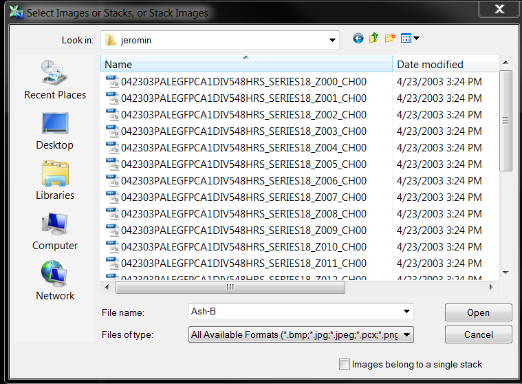
   2. Select files.
      • To select multiple contiguous files, click the first file, hold down the Shift key, click on the last file.
      • To select non-contiguous files, click the first file, hold down the Ctrl key and click to select additional files.
   3. Click Open. The files are added to the list.
   4. Drag a file in the list to change the order of the images (optional).
   5. Click the Next Step button.

3. Specify image scaling.

   1. Specify X Y Scaling

      If needed, update XY scaling information using one of the following methods:

      • Click the From lens radio button and select a lens from the drop-down menu.

      • Click the User defined radio button and enter a value in the X: box.

        Fill in the value for Y by either checking the X=Y checkbox or entering a value in the Y: box.

   2. Specify Z Spacing

      If you are working with 3D images, Z spacing information is needed.

      If needed, update Z spacing by either checking the X=Y=Z checkbox or entering a value in the Z: box.

   3. Click the Next Step button.

4. Define output settings.

   1. Choose the Output File Format by clicking one of the radio buttons:

      • MBF Binary DAT files - can be used with MBF Bioscience products
      • MBF ASC files - compatible with many programs in addition to MBF product

   2. Select the Output Location by clicking a radio button:

      If you choose Another folder, click the Browse button to navigate to and select the destination for your results.

   3. Define Output File Names by clicking a radio button to either:

      • Use image file name with the output file format extension selected above, or

      • Assign a name. Type file name into the box

   4. Click the Next Step button.

5. Trace all files.

   1. Click the Trace All Images button.

      The reconstruction will run and the status bar on the bottom of the 2D window will display progress.

   2. Click the Next Step button.

6. Finish

   Neurolucida 360 software displays a list of data files for the images processed.

   • Double-click a file in the list to load an image and display its trace.
   • Click Open Containing Folder to view single files.

   You can save a log of this session. The log contains information on each image (name, trace file name and location, configuration used, and the trace time) as well as configuration details.